Bulk downloading and analysing MODIS data in R

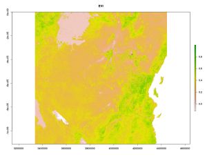
Today we are gonna work with bulk downloaded data from MODIS. The MODIS satellites Terra and Aqua have been floating around the earth since the year 2000 and provide a reliable and free-to-obtain source of remote sensing data for ecologists and conservationists. Among the many MODIS products, Indices of Vegetation Greenness such as NDVI or EVI have been used in countless ecological studies and are the first choice of most ecologists for relating field data to remote sensing data. Here we gonna demonstrate 3 different ways how to acquire and calculate the mean EVI for a given Region and time-period. For this we are using the MOD13Q1 product. We focus on the area a little bit south of Mount Kilimanjaro and the temporal span around May 2014.

(1)
The first handy R-package we gonna use is MODISTools. It is able to download spatial-temporal data via a simple subset command. The nice advantage of using *MODISTools* is that it only downloads the point of interest as the subsetting and processing is done server-wise. This makes it excellent to download only what you need and reduce the amount of download data. A disadvantage is that it queries a perl script on the daac.ornl.gov server, which is often horrible slow and stretched to full capacity almost every second day.

# Using the MODISTools Package
library(MODISTools)
# MODISTools requires you to make a query data.frame
coord <- c(-3.223774, 37.424605) # Coordinates south of Mount Kilimanjaro
product <- "MOD13Q1"
bands <- c("250m_16_days_EVI","250m_16_days_pixel_reliability") # What to query. You can get the names via GetBands
savedir <- "tmp/" # You can save the downloaded File in a specific folder
pixel <- c(0,0) # Get the central pixel only (0,0) or a quadratic tile around it
period <- data.frame(lat=coord[1],long=coord[2],start.date=2013,end.date=2014,id=1)
# To download the pixels
MODISSubsets(LoadDat = period,Products = product,Bands = bands,Size = pixel,SaveDir = "",StartDate = T)
MODISSummaries(LoadDat = period,FileSep = ",", Product = "MOD13Q1", Bands = "250m_16_days_EVI",ValidRange = c(-2000,10000), NoDataFill = -3000, ScaleFactor = 0.0001,StartDate = TRUE,Yield = T,Interpolate = T, QualityScreen = TRUE, QualityThreshold = 0,QualityBand = "250m_16_days_pixel_reliability")
# Finally read the output
read.table("MODIS_Summary_MOD13Q1_2014-08-10.csv",header = T,sep = ",")

The Mean EVI between the year 2013 up to today on the southern slope of Kilimanjaro was .403 (SD=.036). The Yield (integral of interpolated data between start and end date) is 0.05. MODISTools is a very much suitable for you if you want to get hundreds of individual point locations, but less suitable if you want to extract for instance values for a whole area (eg. a polygon shape) or are just annoyed by the frequent server breakdowns…

(2)
If you want to get whole MODIS tiles for your area of interest you have another option in R available. The MODIS package is particularly suited for this job in R and even has options to incorporate ArcGis as path for additional processing. It is also possible to use the MODIS Reprojection Tool or gdal (our choice) as underlying workhorse.

library(MODIS)
dates <- as.POSIXct( as.Date(c("01/05/2014","31/05/2014"),format = "%d/%m/%Y") )
dates2 <- transDate(dates[1],dates[2]) # Transform input dates from before
# The MODIS package allows you select tiles interactively.  We however select them manually here
h = "21"
v = "09"
runGdal(product=product,begin=dates2$beginDOY,end = dates2$endDOY,tileH = h,tileV = v,)
# Per Default the data will be stored in
# ~homefolder/MODIS_ARC/PROCESSED
# After download you can stack the processed TIFS
vi <- preStack(path="~/MODIS_ARC/PROCESSED/MOD13Q1.005_20140810192530/", pattern="*_EVI.tif$")
s <- stack(vi)
s <- s*0.0001 # Rescale the downloaded Files with the scaling factor

# And extract the mean value for our point from before.
# First Transform our coordinates from lat-long to to the MODIS sinus Projection
sp <- SpatialPoints(coords = cbind(coord[2],coord[1]),proj4string = CRS("+proj=longlat +datum=WGS84 +ellps=WGS84"))
sp <- spTransform(sp,CRS(proj4string(s)))
extract(s,sp) # Extract the EVI values for the available two layers from the generated stack
#>  0.2432  | 0.3113

Whole MODIS EVI Tile (250m cs) for East Africa

 

(3)
If all the packages and tools so far did not work as expected, there is also an alternative to use a combination of R and Python to analyse your MODIS files or download your tiles manually. The awesome pyModis scripts allow you to download directly from a USGS server, which at least for me was almost always faster than the LP-DAAC connection the two other solutions before used. However up so far both the MODISTools and MODIS package have processed the original MODIS tiles (which ship in hdf4 container format) for you. Using this solution you have to access the hdf4 files yourself and extract the layers you are interested in.
Here is an example how to download a whole hdf4 container using the modis_download.py script Just query modis_download.py -h if you are unsure about the command line parameters.

# Custom command. You could build your own using a loop and paste
f <- paste0("modis_download.py -r -p MOD13Q1.005 -t ",tile," -e ","2014-05-01"," -f ","2014-05-30"," tmp/","h21v09")
# Call the python script
system(f)
# Then go into your defined download folder (tmp/ in our case)

# Now we are dealing with the original hdf4 files.
# The MODIS package in R has some processing options to get a hdf4 layer into a raster object using gdal as a backbone

library(MODIS)
lay <- "MOD13Q1.A2014145.h21v09.005.2014162035037.hdf" # One of the raw 16days MODIS tiles we downloaded
mod <- getSds(lay,method="gdal") # Get the layer names and gdal links
# Load the layers from the hdf file. Directly apply scaling factor
ndvi <- raster(mod$SDS4gdal[1]) * 0.0001
evi <- raster(mod$SDS4gdal[2]) * 0.0001
reliability <- raster(mod$SDS4gdal[12])
s <- stack(ndvi,evi,reliability)

#Now extract the coordinates values
extract(s,sp)

There you go. Everything presented here was executed on a Linux Debian machine and I have no clue if it works for you Windows or MAC users. Try it out. Hope everyone got some inspiration how to process MODIS data in R 😉