New Paper: Local factors mediate the response of biodiversity to land use on two African mountains

I know that it has been a while since I posted anything here. The daily responsibilities and effort required for my PhD program are taking quite a toll on the time I have available for other non-phd matters (for instance curating this blog). I apologize for this and hope to post some more tutorials and discussion post in the future. However at the moment my personal research reserved 105% of my available time.  But the scientific blogosphere is generally in a bit of a crisis I heard.

Anyway, today I just want to quickly share the exciting news that my MSc thesis I conducted at the Center for Macroecology, Evolution and Climate has passed scientific peer review and is now in early view in Animal Conservation. I am quite proud of this work as it represents the first lead-author paper I managed to publish that involved primary research and data collection.

Short breakdown: During my masters and also now in my PhD I am extensively working with the PREDICTS database, which is a global project aiming at collating local biodiversity estimates in different land-use systems across the entire world. The idea for this work came as I realized that many of the categories in the PREDICTS database are affected by some level of subjectivity. Local factors – such as specific land-use forms, vegetation conditions and species assemblage composition – could alter general responses of biodiversity to land use that have been generalized across larger scales. Thus the simple idea was to compare ‘PREDICTS-style’ model predictions with independent biodiversity estimates raised at the same local scale. But see abstract and paper below.

Jung et al (2016) – Local factors mediate the response of biodiversity to land use on two African mountains

http://onlinelibrary.wiley.com/doi/10.1111/acv.12327/abstract

Abstract:

Land-use change is the single biggest driver of biodiversity loss in the tropics. Biodiversity models can be useful tools to inform policymakers and conservationists of the likely response of species to anthropogenic pressures, including land-use change. However, such models generalize biodiversity responses across wide areas and many taxa, potentially missing important characteristics of particular sites or clades. Comparisons of biodiversity models with independently collected field data can help us understand the local factors that mediate broad-scale responses. We collected independent bird occurrence and abundance data along two elevational transects in Mount Kilimanjaro, Tanzania and the Taita Hills, Kenya. We estimated the local response to land use and compared our estimates with modelled local responses based on a large database of many different taxa across Africa. To identify the local factors mediating responses to land use, we compared environmental and species assemblage information between sites in the independent and African-wide datasets. Bird species richness and abundance responses to land use in the independent data followed similar trends as suggested by the African-wide biodiversity model, however the land-use classification was too coarse to capture fully the variability introduced by local agricultural management practices. A comparison of assemblage characteristics showed that the sites on Kilimanjaro and the Taita Hills had higher proportions of forest specialists in croplands compared to the Africa-wide average. Local human population density, forest cover and vegetation greenness also differed significantly between the independent and Africa-wide datasets. Biodiversity models including those variables performed better, particularly in croplands, but still could not accurately predict the magnitude of local species responses to most land uses, probably because local features of the land management are still missed. Overall, our study demonstrates that local factors mediate biodiversity responses to land use and cautions against applying biodiversity models to local contexts without prior knowledge of which factors are locally relevant.

 

New paper: A first global assessment of remaining biodiversity intactness

Anthropogenic land use is one of the dominant drivers of ongoing biodiversity loss on a global scale and it has often been asked how much biodiversity loss is “too much” for sustaining ecosystem function. Our new paper in the journal Science came out last week and attempts to quantify for the first time the global biodiversity intactness within the planetary boundary framework. I am absolutely delighted to have contributed to this study and it received quite a bit of media attention so far ( https://www.altmetric.com/details/9708902 ) with a number of nice articles in the BBC and the Guardian.

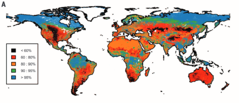
Biodiversity intactness of ecological assemblages for species abundance. Source: Newbold et al. 2016

In our study we calculated the Biodiversity intactness index (BII) first proposed by Scholes and Biggs (2005) for the entire world using the local biodiversity estimates from the PREDICTS project and combined them with the best available down-scaled land-use information to date. We find that many terrestrial biomes are already well beyond the proposed biodiversity planetary boundary (previously defined and set as a precautionary 10% reduction of biodiversity intactness). Unless these ongoing trends are decelerated and stopped in the near future it is likely that biodiversity loss might corroborate national and international biodiversity conservation targets, ecosystem functioning and long-term sustainable development.

• Newbold, Tim, et al. “Has land use pushed terrestrial biodiversity beyond the planetary boundary? A global assessment.” Science 353.6296 (2016): 288-291. DOI: 10.1126/science.aaf2201
• Scholes, R. J., and R. Biggs. “A biodiversity intactness index.” Nature 434.7029 (2005): 45-49. DOI: 10.1038/nature03289

Assessing habitat specialization using IUCN data

Since quite some time ecological models have tried to incorporate both continuous and discrete characteristics of species into their models. Newbold et al. (2013) demonstrated that functional traits affect the response of tropical bird species towards land-use intensity. Tropical forest specialist birds seem to decrease globally in probability of presence and abundance in more intensively used forests. This patterns extends to many taxonomic groups and the worldwide decline of “specialist species” has been noted before by Clavel et al. (2011).

(a) Probabilities of presence of tropical bird species in in different disturbed forests and (b) ratios of abundance in light and intensive disturbed forests relative to undisturbed forests. Forest specialists are disproportionally affected in intensively used forests. Figure from Newbold et al. 2013 doi: http://dx.doi.org/10.1098/rspb.2012.2131

But how to acquire such data on habitat specialization? Ether you assemble your own exhaustive trait database or you query information from some of the openly available data sources. One could for instance be the IUCN redlist, which not only has expert-validated data on a species current threat status, but also on population size and also on a species habitat preference. Here IUCN follows its own habitat classification scheme ( http://www.iucnredlist.org/technical-documents/classification-schemes/habitats-classification-scheme-ver3 ). The curious ecologist and conservationist should keep in mind however, that not all species are currently assessed by IUCN.

There are already a lot of scripts available on the net from which you can get inspiration on how to query the IUCN redlist (Kay Cichini from the biobucket explored this already in 2012 ). Even better: Someone actually compiled a whole r-package called letsR full of web-scraping functions to access the IUCN redlist. Here is some example code for Perrin’s Bushshrike, a tropical bird quite common in central Africa

# Install package
install.packages(letsR)
library(letsR)

# Perrin's or Four-colored Bushshrike latin name
name <- 'Telophorus viridis'

# Query IUCN status
lets.iucn(name)

#>Species        Family Status Criteria Population Description_Year
#>Telophorus viridis MALACONOTIDAE LC Stable 1817
#>Country
#>Angola, Congo, The Democratic Republic of the Congo, Gabon, Zambia

# Or you can query habitat information
lets.iucn.ha(name)

#>Species Forest Savanna Shrubland Grassland Wetlands Rocky areas Caves and Subterranean Habitats
#>Telophorus viridis      1       1         1         0        0           0                               0
#> Desert Marine Neritic Marine Oceanic Marine Deep Ocean Floor Marine Intertidal Marine Coastal/Supratidal
#>      0              0              0                       0                 0                         0
#>  Artificial/Terrestrial Artificial/Aquatic Introduced Vegetation Other Unknown
#>                      1                  0                     0     0       0

letsR also has other methods to work with the spatial data that IUCN provides ( http://www.iucnredlist.org/technical-documents/spatial-data ), so definitely take a look. It works by querying the IUCN redlist api for the species id (http://api.iucnredlist.org/go/Telophorus-viridis). Sadly the habitat function does only return the information if a species is known to occur in a given habitat, but not if it is of major importance for a particular species (so if for instance a Species is known to be a “forest-specialist” ). Telophorus viridis for instance also occurs in savannah and occasionally artificial habitats like gardens ( http://www.iucnredlist.org/details/classify/22707695/0 ).

So I just programmed my own function to assess if forest habitat is of major importance to a given species. It takes a IUCN species id as input and returns ether “Forest-specialist”, if forest habitat is of major importance to a species, “Forest-associated” if a species is just known to occur in forest or “Other Habitats” if a species does not occur in forests at all. The function works be cleverly querying the IUCN redlist and breaking up the HTML structure at given intervals that indicate a new habitat type.

Find the function on gist.github (Strangely WordPress doesn’t include them as they promised)

How does it work? You first enter the species IUCN redlist id. It is in the url after you have queried a given species name. Alternatively you could also download the whole IUCN classification table and match your species name against it 😉 Find it here. Then simply execute the function with the code.

name = 'Telophorus viridis'
data <- read.csv('all.csv')
# This returns the species id
data$Red.List.Species.ID[which(data$Scientific.Name==name)]
#> 22707695

# Then simply run my function
isForestSpecialist(22707695)
#> 'Forest-specialist'

The PREDICTS database: a global database of how local terrestrial biodiversity responds to human impacts

New article in which I am also involved. I have told the readers of the blog about the PREDICTS initiative before. Well, the open-access article describing the last stand of the database has just been released as early-view article. So if you are curious about one of the biggest databases in the world investigating impacts of anthropogenic pressures on biodiversity, please have a look. As we speak the data is used to define new quantitative indices of global biodiversity decline valid for multiple taxa (and not only vertebrates like WWF living planet index).

---

http://onlinelibrary.wiley.com/doi/10.1002/ece3.1303/abstract

Abstract

Biodiversity continues to decline in the face of increasing anthropogenic pressures such as habitat destruction, exploitation, pollution and introduction of alien species. Existing global databases of species’ threat status or population time series are dominated by charismatic species. The collation of datasets with broad taxonomic and biogeographic extents, and that support computation of a range of biodiversity indicators, is necessary to enable better understanding of historical declines and to project – and avert – future declines. We describe and assess a new database of more than 1.6 million samples from 78 countries representing over 28,000 species, collated from existing spatial comparisons of local-scale biodiversity exposed to different intensities and types of anthropogenic pressures, from terrestrial sites around the world. The database contains measurements taken in 208 (of 814) ecoregions, 13 (of 14) biomes, 25 (of 35) biodiversity hotspots and 16 (of 17) megadiverse countries. The database contains more than 1% of the total number of all species described, and more than 1% of the described species within many taxonomic groups – including flowering plants, gymnosperms, birds, mammals, reptiles, amphibians, beetles, lepidopterans and hymenopterans. The dataset, which is still being added to, is therefore already considerably larger and more representative than those used by previous quantitative models of biodiversity trends and responses. The database is being assembled as part of the PREDICTS project (Projecting Responses of Ecological Diversity In Changing Terrestrial Systems – www.predicts.org.uk). We make site-level summary data available alongside this article. The full database will be publicly available in 2015.

---

PS:

I know that I haven’t been particular active on this blog in the last months. I am currently quite busy with writing my Thesis and programming. I am gonna make it up later 🙂

Bulk downloading and analysing MODIS data in R

Today we are gonna work with bulk downloaded data from MODIS. The MODIS satellites Terra and Aqua have been floating around the earth since the year 2000 and provide a reliable and free-to-obtain source of remote sensing data for ecologists and conservationists. Among the many MODIS products, Indices of Vegetation Greenness such as NDVI or EVI have been used in countless ecological studies and are the first choice of most ecologists for relating field data to remote sensing data. Here we gonna demonstrate 3 different ways how to acquire and calculate the mean EVI for a given Region and time-period. For this we are using the MOD13Q1 product. We focus on the area a little bit south of Mount Kilimanjaro and the temporal span around May 2014.

(1)
The first handy R-package we gonna use is MODISTools. It is able to download spatial-temporal data via a simple subset command. The nice advantage of using *MODISTools* is that it only downloads the point of interest as the subsetting and processing is done server-wise. This makes it excellent to download only what you need and reduce the amount of download data. A disadvantage is that it queries a perl script on the daac.ornl.gov server, which is often horrible slow and stretched to full capacity almost every second day.

# Using the MODISTools Package
library(MODISTools)
# MODISTools requires you to make a query data.frame
coord <- c(-3.223774, 37.424605) # Coordinates south of Mount Kilimanjaro
product <- "MOD13Q1"
bands <- c("250m_16_days_EVI","250m_16_days_pixel_reliability") # What to query. You can get the names via GetBands
savedir <- "tmp/" # You can save the downloaded File in a specific folder
pixel <- c(0,0) # Get the central pixel only (0,0) or a quadratic tile around it
period <- data.frame(lat=coord[1],long=coord[2],start.date=2013,end.date=2014,id=1)
# To download the pixels
MODISSubsets(LoadDat = period,Products = product,Bands = bands,Size = pixel,SaveDir = "",StartDate = T)
MODISSummaries(LoadDat = period,FileSep = ",", Product = "MOD13Q1", Bands = "250m_16_days_EVI",ValidRange = c(-2000,10000), NoDataFill = -3000, ScaleFactor = 0.0001,StartDate = TRUE,Yield = T,Interpolate = T, QualityScreen = TRUE, QualityThreshold = 0,QualityBand = "250m_16_days_pixel_reliability")
# Finally read the output
read.table("MODIS_Summary_MOD13Q1_2014-08-10.csv",header = T,sep = ",")

The Mean EVI between the year 2013 up to today on the southern slope of Kilimanjaro was .403 (SD=.036). The Yield (integral of interpolated data between start and end date) is 0.05. MODISTools is a very much suitable for you if you want to get hundreds of individual point locations, but less suitable if you want to extract for instance values for a whole area (eg. a polygon shape) or are just annoyed by the frequent server breakdowns…

(2)
If you want to get whole MODIS tiles for your area of interest you have another option in R available. The MODIS package is particularly suited for this job in R and even has options to incorporate ArcGis as path for additional processing. It is also possible to use the MODIS Reprojection Tool or gdal (our choice) as underlying workhorse.

library(MODIS)
dates <- as.POSIXct( as.Date(c("01/05/2014","31/05/2014"),format = "%d/%m/%Y") )
dates2 <- transDate(dates[1],dates[2]) # Transform input dates from before
# The MODIS package allows you select tiles interactively.  We however select them manually here
h = "21"
v = "09"
runGdal(product=product,begin=dates2$beginDOY,end = dates2$endDOY,tileH = h,tileV = v,)
# Per Default the data will be stored in
# ~homefolder/MODIS_ARC/PROCESSED
# After download you can stack the processed TIFS
vi <- preStack(path="~/MODIS_ARC/PROCESSED/MOD13Q1.005_20140810192530/", pattern="*_EVI.tif$")
s <- stack(vi)
s <- s*0.0001 # Rescale the downloaded Files with the scaling factor

# And extract the mean value for our point from before.
# First Transform our coordinates from lat-long to to the MODIS sinus Projection
sp <- SpatialPoints(coords = cbind(coord[2],coord[1]),proj4string = CRS("+proj=longlat +datum=WGS84 +ellps=WGS84"))
sp <- spTransform(sp,CRS(proj4string(s)))
extract(s,sp) # Extract the EVI values for the available two layers from the generated stack
#>  0.2432  | 0.3113

Whole MODIS EVI Tile (250m cs) for East Africa

 

(3)
If all the packages and tools so far did not work as expected, there is also an alternative to use a combination of R and Python to analyse your MODIS files or download your tiles manually. The awesome pyModis scripts allow you to download directly from a USGS server, which at least for me was almost always faster than the LP-DAAC connection the two other solutions before used. However up so far both the MODISTools and MODIS package have processed the original MODIS tiles (which ship in hdf4 container format) for you. Using this solution you have to access the hdf4 files yourself and extract the layers you are interested in.
Here is an example how to download a whole hdf4 container using the modis_download.py script Just query modis_download.py -h if you are unsure about the command line parameters.

# Custom command. You could build your own using a loop and paste
f <- paste0("modis_download.py -r -p MOD13Q1.005 -t ",tile," -e ","2014-05-01"," -f ","2014-05-30"," tmp/","h21v09")
# Call the python script
system(f)
# Then go into your defined download folder (tmp/ in our case)

# Now we are dealing with the original hdf4 files.
# The MODIS package in R has some processing options to get a hdf4 layer into a raster object using gdal as a backbone

library(MODIS)
lay <- "MOD13Q1.A2014145.h21v09.005.2014162035037.hdf" # One of the raw 16days MODIS tiles we downloaded
mod <- getSds(lay,method="gdal") # Get the layer names and gdal links
# Load the layers from the hdf file. Directly apply scaling factor
ndvi <- raster(mod$SDS4gdal[1]) * 0.0001
evi <- raster(mod$SDS4gdal[2]) * 0.0001
reliability <- raster(mod$SDS4gdal[12])
s <- stack(ndvi,evi,reliability)

#Now extract the coordinates values
extract(s,sp)

There you go. Everything presented here was executed on a Linux Debian machine and I have no clue if it works for you Windows or MAC users. Try it out. Hope everyone got some inspiration how to process MODIS data in R 😉

It is conference-summer – BES-TEG in YORK 2014

The Sun is shining, birds are singing and most scientists have nothing better to do than jetting around the globe to attend conferences. Yes, it is summer indeed. Here is some advertising for the 2014 Tropical Ecology – Early Carer Meeting of the British Ecological Society. This year the fun is happening in York. As many people seem to be on vacation the deadline for abstracts has been extended to the 14th of July. See the attached Documents ( BES-TEG 2014 Flyer ,BES_TEG Key speakers ) for more information. I will be there as well… .

---

Dear All,

The British Ecology Society – Tropical Ecology Group (BES-TEG) are organizing a 7th early career meeting scheduled to take place at the University of York, on the 14th and 15th of August 2014. Day one will focus on Ecology and Ecosystem Processes while day two will focus on Practical Applications and Links to Policy; such as conservation, livelihood, policy and development. All early-career researchers, both PhD and Post-Docs, are welcome to present their tropical ecology related research as a poster and/or oral presentation. The deadline for abstract submission has been extended to Monday the 14th of July 2014.

Please find attached the flyer and conference document for detailed information.

It would be appreciated if this flyer circulates within your department. Students are encouraged to come to York for what should be a really interesting few days in August.

An event website has been set up for registration

http://www.eventbrite.co.uk/o/british-ecological-society-tropical-ecology-group-bes-teg-6217007537

Interesting Paper: Global warming and invertebrate colouring

Just now another very interesting paper has been published in Nature Communications, which was written by former colleagues of mine from the University of Marburg.

Global warming favours light-coloured insects in Europe

As we all know many insect species like butterflies, bees or dragonflies have their main activity pattern during the day due to their ectotherm thermoregulation. Body colour is an important aspect of this thermoregulation as darker ( more blackish) individuals usually heat up faster. Therefore darker insects have an advantage compared to brighter insects in cooler climates as they heat up more rapidly and can forage earlier. This pattern can be mapped on a larger scale using occurrence data and has been known as “thermal melanism hypothesis” in macroecology. The authors go a step further from here as they  not only display a new biogeographic pattern previously unknown to science ( colouring gradient of European dragonflies and butterflies from south to north), but they also demonstrate how this mechanistic link between a macroecological pattern and a functional trait can be used to forecast the effect of climate change on insects.

From Zeuss et al. (2014): Shift in colour value for (a) the raw data; (b) the phylogenetic component (P); and (c) the specific component (S). Red indicates an increase in colour lightness; blue indicates a decrease in colour lightness. The diameter of each dot indicates the extent of the shift (n=1,845). The distribution of the shifts shows for the specific component a clear trend towards higher (that is, lighter-coloured) values (peak of the distribution positive; zero indicated by black line). The phylogenetic component suggests that the shifts in colour lightness have a strong phylogenetic background leading to a complex geographic mosaic in the response of assemblages to climate change. The inserted histograms show the mean change in colour lightness calculated for 1,000 alternative phylogenetic trees and are positive throughout, indicating that uncertainties in the phylogenetic hypotheses are unlikely to affect our conclusion of a general shift towards lighter assemblages. The distributional information used in the analysis is often based on a large time span, that is, the distributional information published in 1988 summarizes data until that year using information even from the beginning of the twentieth century. Rugs at the abscissa indicate observed values.

Possible critics: A definite next step in the analysis would be to include real measurements of optical colour rather than RGB values of scanned pictures. The colour values used in this study were all derived from scientific taxonomic drawings of those insects and thus biased by subjectivity of the respective artist. Nevertheless this bias should be consistent (if the same artist has sketched the images) so it should not influence the colouring gradient.  It is also interesting to note that many insects ( I know this for instance from my work with bugs and hoverflies) can adapt their body colouring to their habitat or differ quite a lot within a population. Differing melanism in body color and wing colouration might be related to the climatic niche they occur in, but the insects themselves might also possess phenotypic plasticity to adapt for instance to different habitats and background (Hochkirch et al. 2008). This pattern certainly needs more investigations in the future.

The article has been published as open access paper, so give it a try 😉

• Hochkirch, A., Deppermann, J. and Gröning, J. (2008), Phenotypic plasticity in insects: the effects of substrate color on the coloration of two ground-hopper species. Evolution & Development, 10: 350–359.

• Zeuss, D. et al. (2014) Global warming favours light-coloured insects in Europe. Nat. Commun. 5:3874

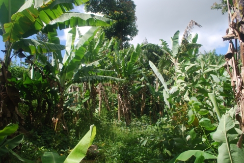
Out in the field – Working in the agricultural Mosaic of the Taita Hills

And here are some news from my current field work that is part of my Thesis. After spending some quiet, but exiting days in Nairobi (maybe later more about that) I finally arrived in Wundanyi, Taita Hills, where a substantial part of my work will be conducted along the CHIESA transect. Suited in the coastel area in proximity to Mombasa the Taita Hills are renown for their extraordinary bird diversity and endemic species and as such are considered to be part of the Eastern Arc Mountains Diversity hotspot. The Taita hills encompass a variety of different land-use forms, but the majority of them surely are tropical homegardens as most of the “Taita” people are subsistence farmers growing crops in the highly fertile soil of the mountain slopes. Besides homegardens there are riverine forests in the valleys, shrubland vegetation in the lower altitudes, exotic tree plantations and of course the remaining indigenous forests remaining on the Taita hills mountain tops. Every last forest part is known well and was traditionally protected by the locals as part of their culture. However in the later centuries the remaining forest area became more and more scarcer and even during my visits in some of the forest fragments with the highest biodiversity value (Chawia, Ngangao) I saw frequent signs of fuelwood and timber extraction. Clearly a lack of funding for biodiversity protection seems to be the problem, but also an economic perspective and opportunities such as ecotourism might enhance locals perception if and how these last forest parts should be protected.

Past Funding

Cloud Forest Vuria

Woodland

My work in the Taita hills is all about birds. Specifically I am conducting avian diversity and abundance assessments along an altitudinal transect encompassing a variety of different land-use systems. Although avian assessments have been conducted in Taita many times before, they were often restricted to the forest fragments and for instance didn’t look at the bird diversity in homegardens in different altitudes. The resulting data will just be used for my thesis as validation dataset, but I am hoping that it has maybe some value on its own as well. Initial results show that especially the homegarden in Taita support quite a high diversity of birds, which is even similar to levels in the remaining forest fragments (although the community is somewhat different and biotic homogenization is likely on-going).

It can be quite challenging to conduct avian research in tropical human-dominated landscapes. Not only do you have to arrange for transport to the specific transect areas and lodging (in my case provided by the University of Helsinki Research station in Wundanyi), but also account for the frequent interruption by children and farmers asking what you are doing. Furthermore it is not an easy task to count birds in for instance a maize or sugarcane plantation due to the limited accessibility and my intention not to damage the farmers crops. Most of the farmers however happily provide access to their land and are very interested in what kind of research this “Mzungu” is doing on their farm. From my own experience here I can tell that the Taita people are very kind and it is a pleasure to work with them on their land. They are very respectful and even walking around late at night or very early in the morning seems to be no problem here (in contrast to for instance Nairobi or Mombasa).

Speckled Mousebird

Female Chameleon

In the end my sampling goes on quite well and much better than I expected. Although it is technically raining season and long heavy rains can be expected every day, the mornings were exceptionally dry and weather was mostly favourable for ornithological research. Generally this time of the year in East Africa is especially interesting for bird assessments as many local bird species are in their breeding plumage and nesting, but also because European migrants are often still around or on their way back to Europe (for instance I saw and heard an European Willow Warbler some days ago). Lets see what else the next weeks will have for be in terms of avian diversity.

The PREDICTS project – We need your data!

As part of my Thesis project I have recently joined up with the researchers and interns of the PREDICTS project. PREDICTS stands for Projecting Responses of Ecological Diversity In Changing Terrestrial Systems (yeah, fancy and down-to-the-point acronym) and is aiming to investigate the impact of various human pressures on biological diversity on a global scale. PREDICTS gets its data from contributing authors and is constantly looking for new data contributors. All contributors will become coauthors of a paper describing the database and  at the end of the project the whole database will be released to the public!

We want your data! For instance Wildcat (Felis sylvestris) encounters in different habitat types!

If you have diversity or community composition data collected from more than one terrestrial site which are somehow influenced by humanity and are raised using a standardized methodology, then it is more than likely that we could use it. What we need is the

• Locations of sampling points, as precisely as possible
  (with the coordinate system used, if possible)
• An indication of the type of land cover that each sampling point represents
  (e.g. primary forest, secondary forest, intensively-farmed crop, hedgerow)
• An indication of how intensively the site is used by people
• Data on the presence / absence, or ideally a measure of abundance, of each species at each site
• The date(s) that each measurement was taken

We need more openness in terms of data sharing in conservation and ecology research! It is unbelievable that some important research data even today can go lost if for instance the original author died or his lab burned to the ground. Some might argue that it should be mandatory to share data if your research is 100% funded by public sources. Some understandable reasons that speak against data sharing after publication are for instance that you are a young emerging scientist and want to keep your hardly earned golden eggs to yourself. However this can be debated as well as data sharing not only gives you more citations, but maybe even into contact with other researchers in your field. In other cases researchers sometimes don’t want to share raw sampling data because of conservation concerns, but even here there are options to coarsen coordinates before public release.

Recent initiatives on openness in terms of ecological data sharing like https://datadryad.org/ and http://figshare.com/ already provide a splendid place where you as an Author can dump raw data from papers you wrote years ago. You can even place the raw data from your most current projects and put an embargo on the download so that the item will be released to the public for instance one year after the associated article has been published.

Anyway:

For my thesis I am especially looking for all kinds of African community data that has been published. We already have a lot of studies in the database, but for my project i need more data especially of less sampled taxa (insects, amphibians,…), different temporal resolutions and a greater diversity of land-use types.  So especially if you have data on African species communities in any form (diversity metrics, abundance metrics, I even take occurence matrices) which were sampled in somehow anthropogenic disturbed habitats: Please contact me or wait for me to contact you 🙂

Martin Jung

Macroecology playground (3) – Spatial autocorrelation

Hey, it has been over 2 months, so welcome in 2014 from my side. And i am sorry for not posting more updates recently, but like everyone i was (and still am) under constant working pressure. This year will be quite interesting for me personally as i am about to start my thesis project and will (besides other things) go to Africa for fieldwork. But for now i will try to catch your interest with a new macroecology playground post dealing with the important issue of spatial autocorrelation. See the other Macroecology playground posts here and here for knowing what happened in the past.

---

Spatial autocorrelation is the issue that data points in geographical space are somewhat dependent on each other or their values correlated because of spatial proximity/distance. This is also known as the first law of geography (Google it). However, most of the statistical tools we have available assume that all our datapoints are independent from each other, which is rarely the case in macroecology. Just imagine the steep slope of mountain regions. Literally all big values will always occur near the peak of the mountains and decrease with distance from the peak. There is thus already a data-inherent gradient present which we somehow have to account for, if we are to investigate the effect of altitude alone (and not the effect of the proximity to nearby cells).

In our hypothetical example we want to explore how well the topographical average (average height per grid cell) can explain amphibian richness in South America and if the residuals (model errors) in our model are spatially autocorrelated. I can’t share the data, but i believe the dear reader will get the idea of what we are trying to do.

# Load libraries
library(raster)

# Load in your dataset. In my case i am loading both the Topo and richness from a raster stack.
amp <- s$Amphibians.richness
topo <- s$Topographical.Average
summary(fit1 <- lm(getValues(amp)~getValues(topo)))
# Extract from the output
Multiple R-squared: 0.1248, Adjusted R-squared: 0.1242
F-statistic: 217.7 on 1 and 1527 DF, p-value: < 2.2e-16

par(mfrow=c(2,1))
plot(amp,col=rainbow(100,start=0.2))
plot(s$Topographical.Average)

What did we do? As you can see we fitted a simple linear regression model using the values from both the amphibian richness raster layer and the topographical range raster. The relation seems to be highly significant and this simple model can explain up to 12.4% of the variation. Here is the basic plot output for both response and predictor variable.

Plot of response and predictor values

As you can see high values of both layers seem to be spatially clustered. So the likelihood of violating the independence of datapoints in a linear regression model is quite likely. Lets investigate the spatial autocorrelation by looking at Moran’s I, which is a measure for spatial autocorrelation (technically its just a determinant of correlation that calculated the pearsons r of surrounding values within a certain window). So lets investigate if the residual values (the error in model fit) are spatially autocorrelated.

library(ncf) # For the Correlogram

# Generate an Residual Raster from the model before
rval <- getValues(amp) # Create new raster
rval[as.numeric(names(fit1$residuals))]<- fit1$residuals # replace all data-cells with res value
resid <- topo
values(resid) <-rval;rm(rval) #replace our values in this new raster
names(resid) <- "Residuals"

# Now calculate Moran's I of the new residual raster layer
x = xFromCell(resid,1:ncell(resid)) # take x coordinates
y = yFromCell(resid,1:ncell(resid)) # take y coordinates
z = getValues(resid) # and the values of course
# Now calculate Moran's I
# Use the extracted coordinates and values, increase the distance in 100er steps and don't forget to use latlon=T (given that you have your rasters in WGS84 projected)
system.time(co <- correlog(x,y,z,increment = 100,resamp = 0, latlon = T,na.rm=T)) # this can take a while.
# It takes even longer if you try to estimate significance of spatial autocorrelation

# Now show the result
plot(0,type="n",col="black",ylab="Moran's I",xlab="lag distance",xlim=c(0,6500),ylim=c(-1,1))
abline(h=0,lty="dotted")
lines(co$correlation~co$mean.of.class,col="red",lwd=2)
points(x=co$x.intercept,y=0,pch=19,col="red")

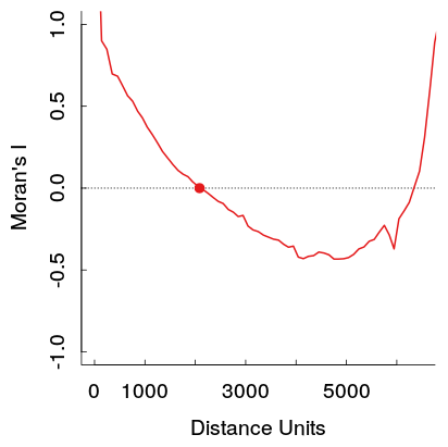
Moran’s I of the model residuals

Ideally Moran’s I should be as close to zero as possible. In the above plot you can see that values in close distance (up to 2000 Distance units) and with greater distance as well, the model residuals are positively autocorrelated (too great than expected by chance alone, thus correlated with proximity). The function correlog allows you to resample the dataset to investigate significance of this patterns, but for now i will just assume that our models residuals are significantly spatially autocorrelated.

There are numerous techniques to deal with or investigate spatial autocorrelation. Here the interested reader is advised to look at Dormann et al. (2007) for inspiration. In our example we will try to fit a simultaneous spatial autoregressive model (SAR) and try to see if we can partially get the spatial autocorrelation out of the residual error.  SARs can model the spatial error generating process and operate with weight
matrices that specify the strength of interaction between neighbouring sites (Dormann et al., 2007). If you know that the spatial autocorrelation occurs in the response variable only, a so called “lagged-response model” would be most appropriate, otherwise use a “mixed” SAR if the error occurs in both response and predictors. However Kissling and Carl (2008) investigated SAR models in detail and came to the conclusion that lagged and mixed SARs might not always give better results than ordinary least square regressions and can generate bias (Kissling & Carl, 2008). Instead they recommend to calculate “spatial error” SAR models when dealing with species distribution data, which assumes that the spatial correlation does neither occur in response or predictors, but in the error term.

So lets build the spatial weights and fit a SAR:

library(spdep)

x = xFromCell(amp,1:ncell(amp))
y = yFromCell(amp,1:ncell(amp))
z = getValues(amp)
nei <- dnearneigh(cbind(x,y),d1=0,d2=2000,longlat=T) # Get neighbourlist of interactions with a distance unit 2000.
nlw <- nb2listw(nei,style="W",zero.policy=T)
# You should calculate the interaction weights with the maximal distance in which autocorrelation occurs.
# But here we will just take the first x-intercept where positive correlation turns into the negative.
# Now fit the spatial error SAR
sar_e <- errorsarlm(z~topo,data=val,listw=nlw,na.action=na.omit,zero.policy=T)
# We use the generated z values and weights as input. Nodata values are excluded and zeros are given to boundary errors

# Now compare how much Variation can be explained
summary(fit1)$adj.r.squared # The r_squared of the normal regression
> 0.124
summary(sar_e,Nagelkerke=T)$NK # Nagelkerkes pseudo r_square of the SAR
> 0.504 # -- for SAR. So we could increase the influence of topographical average value on amphibian richness

# Finally do a likelihood ratio test
LR.sarlm(sar_e,fit1)
# Likelihood ratio for spatial linear models
>data:
>Likelihood ratio = 869.7864, df = 1, p-value &lt; 2.2e-16
>sample estimates:
>Log likelihood of sar_e; Log likelihood of fit1
> -7090.903 
>-7525.796

# Not only are our two models significantly different, but the log likelihood of our SAR is also greater than the ordinary model
# indicating a better fit.

The SAR is one of many methods to deal with spatial autocorrelation. I agree that the choice of of the weights matrix distance is a bit arbitrary (it made sense for me), so you might want to investigate the occurence of spatial correlations a bit more prior to fitting a SAR. So have we dealt with the autocorrelation? Lets just calculate Moran’s I values again for both the old residual and the SAR residual values. Looks better doesn’t it?

Comparison of Moran’s I for both a linear model and a error SAR residuals

References:

• F Dormann, C., M McPherson, J., B Araújo, M., Bivand, R., Bolliger, J., Carl, G., … & Wilson, R. (2007). Methods to account for spatial autocorrelation in the analysis of species distributional data: a review. Ecography, 30(5), 609-628.
• Kissling, W. D., & Carl, G. (2008). Spatial autocorrelation and the selection of simultaneous autoregressive models. Global Ecology and Biogeography, 17(1), 59-71.