New Paper: Local factors mediate the response of biodiversity to land use on two African mountains

I know that it has been a while since I posted anything here. The daily responsibilities and effort required for my PhD program are taking quite a toll on the time I have available for other non-phd matters (for instance curating this blog). I apologize for this and hope to post some more tutorials and discussion post in the future. However at the moment my personal research reserved 105% of my available time.  But the scientific blogosphere is generally in a bit of a crisis I heard.

Anyway, today I just want to quickly share the exciting news that my MSc thesis I conducted at the Center for Macroecology, Evolution and Climate has passed scientific peer review and is now in early view in Animal Conservation. I am quite proud of this work as it represents the first lead-author paper I managed to publish that involved primary research and data collection.

Short breakdown: During my masters and also now in my PhD I am extensively working with the PREDICTS database, which is a global project aiming at collating local biodiversity estimates in different land-use systems across the entire world. The idea for this work came as I realized that many of the categories in the PREDICTS database are affected by some level of subjectivity. Local factors – such as specific land-use forms, vegetation conditions and species assemblage composition – could alter general responses of biodiversity to land use that have been generalized across larger scales. Thus the simple idea was to compare ‘PREDICTS-style’ model predictions with independent biodiversity estimates raised at the same local scale. But see abstract and paper below.

Jung et al (2016) – Local factors mediate the response of biodiversity to land use on two African mountains

http://onlinelibrary.wiley.com/doi/10.1111/acv.12327/abstract

Abstract:

Land-use change is the single biggest driver of biodiversity loss in the tropics. Biodiversity models can be useful tools to inform policymakers and conservationists of the likely response of species to anthropogenic pressures, including land-use change. However, such models generalize biodiversity responses across wide areas and many taxa, potentially missing important characteristics of particular sites or clades. Comparisons of biodiversity models with independently collected field data can help us understand the local factors that mediate broad-scale responses. We collected independent bird occurrence and abundance data along two elevational transects in Mount Kilimanjaro, Tanzania and the Taita Hills, Kenya. We estimated the local response to land use and compared our estimates with modelled local responses based on a large database of many different taxa across Africa. To identify the local factors mediating responses to land use, we compared environmental and species assemblage information between sites in the independent and African-wide datasets. Bird species richness and abundance responses to land use in the independent data followed similar trends as suggested by the African-wide biodiversity model, however the land-use classification was too coarse to capture fully the variability introduced by local agricultural management practices. A comparison of assemblage characteristics showed that the sites on Kilimanjaro and the Taita Hills had higher proportions of forest specialists in croplands compared to the Africa-wide average. Local human population density, forest cover and vegetation greenness also differed significantly between the independent and Africa-wide datasets. Biodiversity models including those variables performed better, particularly in croplands, but still could not accurately predict the magnitude of local species responses to most land uses, probably because local features of the land management are still missed. Overall, our study demonstrates that local factors mediate biodiversity responses to land use and cautions against applying biodiversity models to local contexts without prior knowledge of which factors are locally relevant.

 

Android apps for researchers – My personal favourites

For a long time I have been kinda reluctant to jump on the Smartphone/Touchscreen train, which might be due to the fact that I am rather conservative with regards to software. In the same way I choose my Linux distribution (Debian for the extra stability and often outdated , but proofed versions), I prefer to choose the tools surrounding me. Stability and function always meant a lot more to me than cultural trends or taste. Nevertheless in the last month I decided to purchase my first device with a touchscreen, a tablet running Android for my daily use and so that I do not have to take the notebook with me during every travel. I have never really used sth. like this before so please excuse the following over exaggerated praises as this whole world of using apps (as in application) is pretty new to me. In the short time I used my new tabet, I already managed to find some really useful apps, which I would like to share with you (feel free to recommend others):

• Browzine

Doing any kind of research usually requires you to read broadly and read a lot! Most of the time I stumble across new literature by reading blogs, tweets and following researchers who work on similar issues related to mine. Of course I occasionally check out different journal homepages as well and scroll down the list of abstracts from the latest issues. Working or being registered at a scientific institution enables you to read papers from all kinds of journals, not only those directly related to your main field of research. I promptly registered to many journals including some that are only in a very general way related to my field of study. In Browzine published new issues are highlighted with a red dot, so you can be sure never to miss a new paper from your favourite journal. In addition you can save any downloaded papers directly to your dropbox or mendeley account. Cons: Some opensource journals (peerJ) and preprint hosters (biorxiv) are missing? Also it seems as if not every institution has made a deal with the app publisher.

• Evernote

This one probably is not a new one to you. Evernote has been around for a while and simply does a splendid job of organizing your thoughts. You can drop whole websites, simple txt’s and pictures together to build your own little collection of paste-it posts. I usually also keep their web interface open on my desktop PC and all notes are synchronized with my mobile device.

• Mendeley

If you are not running windows / evernote on your production machine, than usually you go with ether Zotero or mendeley as literature management software of your choice. I got used to mendeley and their nice plugin for Libreoffice, which enables to insert and manage references directly from mendeley. This really paid off when I noticed that there is also a mendeley app, which syncs with your mendeley account. Why is that useful? Well, I can for instance manage all my references and tons of pdfs on my PC, sync them to my mendeley account and then have them readily available for reading and commenting on my mobile device. Not to mention that it integrates quite well with other providers such as the mentioned above Browzine.

• ES File Explorer

Excellent file browser which I really would like to have open all the time. You can browse all the files on your device (even the hidden once), social and remote service (like cloud hoster, ftp or network servers) are integrated. The ES File explorer is organized in windows, which enables you to switch quickly between for instance your dropbox and pictures. Very good discovery!

• Google calendar and mail

I tried almost every calender and mail app that is available in the google play store, but in the end I still stuck with the default google calendar and mail. The reasons: Ease of navigations, no annoying adds or popups which want to persuade you to buy a “pro” version and especially working sync with a wide range of accounts, contacts and events(!). Obviously the google apps have kinda of a homeplay game on android compared to other alternatives. Having the same kind of interface for the calendar on both the tablet and my personal computer was really, what made the deal in the end. Google mail also is quite easy to use and manage, especially for people like me with multiple mail accounts.

• OsmAnd

This one is really handy, especially for people who often get lost. It lets you access the popular openstreemap maps and navigate through it with your touchscreen. If you enable GPS you can see your current location and calculate the optimal route to your destination. Out of internet? No problem, the app lets you download and store whole geographic regions so that you can access openstreetmaps mapping and routing even while you are have no internet. Quite good if you are lost on the way to a conference and don’t want to use your precious bandwidth.

• Map of Life

This one is an output from the Jetz lab at Yale university. You can use the application to find out the species that you just saw on your morning stroll around the park/coast/reserve. Based on species range maps it calculates the number of species, which can be potentially discovered in the current area. The little pictures also help a lot with the identification.

That´s it. But feel welcome to comment and suggest other nice (free) apps. I should explicitly mention that I am not related or employed by any of the apps´s providers.

Out in the field – Working in the agricultural Mosaic of the Taita Hills

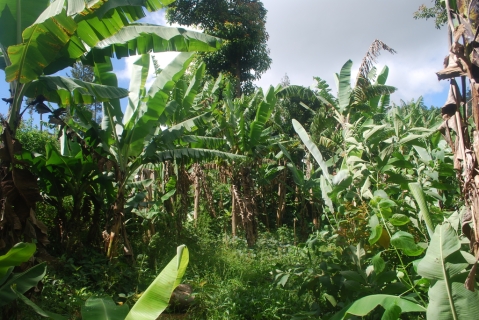
And here are some news from my current field work that is part of my Thesis. After spending some quiet, but exiting days in Nairobi (maybe later more about that) I finally arrived in Wundanyi, Taita Hills, where a substantial part of my work will be conducted along the CHIESA transect. Suited in the coastel area in proximity to Mombasa the Taita Hills are renown for their extraordinary bird diversity and endemic species and as such are considered to be part of the Eastern Arc Mountains Diversity hotspot. The Taita hills encompass a variety of different land-use forms, but the majority of them surely are tropical homegardens as most of the “Taita” people are subsistence farmers growing crops in the highly fertile soil of the mountain slopes. Besides homegardens there are riverine forests in the valleys, shrubland vegetation in the lower altitudes, exotic tree plantations and of course the remaining indigenous forests remaining on the Taita hills mountain tops. Every last forest part is known well and was traditionally protected by the locals as part of their culture. However in the later centuries the remaining forest area became more and more scarcer and even during my visits in some of the forest fragments with the highest biodiversity value (Chawia, Ngangao) I saw frequent signs of fuelwood and timber extraction. Clearly a lack of funding for biodiversity protection seems to be the problem, but also an economic perspective and opportunities such as ecotourism might enhance locals perception if and how these last forest parts should be protected.

Past Funding

Cloud Forest Vuria

Woodland

My work in the Taita hills is all about birds. Specifically I am conducting avian diversity and abundance assessments along an altitudinal transect encompassing a variety of different land-use systems. Although avian assessments have been conducted in Taita many times before, they were often restricted to the forest fragments and for instance didn’t look at the bird diversity in homegardens in different altitudes. The resulting data will just be used for my thesis as validation dataset, but I am hoping that it has maybe some value on its own as well. Initial results show that especially the homegarden in Taita support quite a high diversity of birds, which is even similar to levels in the remaining forest fragments (although the community is somewhat different and biotic homogenization is likely on-going).

It can be quite challenging to conduct avian research in tropical human-dominated landscapes. Not only do you have to arrange for transport to the specific transect areas and lodging (in my case provided by the University of Helsinki Research station in Wundanyi), but also account for the frequent interruption by children and farmers asking what you are doing. Furthermore it is not an easy task to count birds in for instance a maize or sugarcane plantation due to the limited accessibility and my intention not to damage the farmers crops. Most of the farmers however happily provide access to their land and are very interested in what kind of research this “Mzungu” is doing on their farm. From my own experience here I can tell that the Taita people are very kind and it is a pleasure to work with them on their land. They are very respectful and even walking around late at night or very early in the morning seems to be no problem here (in contrast to for instance Nairobi or Mombasa).

Speckled Mousebird

Female Chameleon

In the end my sampling goes on quite well and much better than I expected. Although it is technically raining season and long heavy rains can be expected every day, the mornings were exceptionally dry and weather was mostly favourable for ornithological research. Generally this time of the year in East Africa is especially interesting for bird assessments as many local bird species are in their breeding plumage and nesting, but also because European migrants are often still around or on their way back to Europe (for instance I saw and heard an European Willow Warbler some days ago). Lets see what else the next weeks will have for be in terms of avian diversity.

The PREDICTS project – We need your data!

As part of my Thesis project I have recently joined up with the researchers and interns of the PREDICTS project. PREDICTS stands for Projecting Responses of Ecological Diversity In Changing Terrestrial Systems (yeah, fancy and down-to-the-point acronym) and is aiming to investigate the impact of various human pressures on biological diversity on a global scale. PREDICTS gets its data from contributing authors and is constantly looking for new data contributors. All contributors will become coauthors of a paper describing the database and  at the end of the project the whole database will be released to the public!

We want your data! For instance Wildcat (Felis sylvestris) encounters in different habitat types!

If you have diversity or community composition data collected from more than one terrestrial site which are somehow influenced by humanity and are raised using a standardized methodology, then it is more than likely that we could use it. What we need is the

• Locations of sampling points, as precisely as possible
  (with the coordinate system used, if possible)
• An indication of the type of land cover that each sampling point represents
  (e.g. primary forest, secondary forest, intensively-farmed crop, hedgerow)
• An indication of how intensively the site is used by people
• Data on the presence / absence, or ideally a measure of abundance, of each species at each site
• The date(s) that each measurement was taken

We need more openness in terms of data sharing in conservation and ecology research! It is unbelievable that some important research data even today can go lost if for instance the original author died or his lab burned to the ground. Some might argue that it should be mandatory to share data if your research is 100% funded by public sources. Some understandable reasons that speak against data sharing after publication are for instance that you are a young emerging scientist and want to keep your hardly earned golden eggs to yourself. However this can be debated as well as data sharing not only gives you more citations, but maybe even into contact with other researchers in your field. In other cases researchers sometimes don’t want to share raw sampling data because of conservation concerns, but even here there are options to coarsen coordinates before public release.

Recent initiatives on openness in terms of ecological data sharing like https://datadryad.org/ and http://figshare.com/ already provide a splendid place where you as an Author can dump raw data from papers you wrote years ago. You can even place the raw data from your most current projects and put an embargo on the download so that the item will be released to the public for instance one year after the associated article has been published.

Anyway:

For my thesis I am especially looking for all kinds of African community data that has been published. We already have a lot of studies in the database, but for my project i need more data especially of less sampled taxa (insects, amphibians,…), different temporal resolutions and a greater diversity of land-use types.  So especially if you have data on African species communities in any form (diversity metrics, abundance metrics, I even take occurence matrices) which were sampled in somehow anthropogenic disturbed habitats: Please contact me or wait for me to contact you 🙂

Martin Jung

Macroecology playground (3) – Spatial autocorrelation

Hey, it has been over 2 months, so welcome in 2014 from my side. And i am sorry for not posting more updates recently, but like everyone i was (and still am) under constant working pressure. This year will be quite interesting for me personally as i am about to start my thesis project and will (besides other things) go to Africa for fieldwork. But for now i will try to catch your interest with a new macroecology playground post dealing with the important issue of spatial autocorrelation. See the other Macroecology playground posts here and here for knowing what happened in the past.

---

Spatial autocorrelation is the issue that data points in geographical space are somewhat dependent on each other or their values correlated because of spatial proximity/distance. This is also known as the first law of geography (Google it). However, most of the statistical tools we have available assume that all our datapoints are independent from each other, which is rarely the case in macroecology. Just imagine the steep slope of mountain regions. Literally all big values will always occur near the peak of the mountains and decrease with distance from the peak. There is thus already a data-inherent gradient present which we somehow have to account for, if we are to investigate the effect of altitude alone (and not the effect of the proximity to nearby cells).

In our hypothetical example we want to explore how well the topographical average (average height per grid cell) can explain amphibian richness in South America and if the residuals (model errors) in our model are spatially autocorrelated. I can’t share the data, but i believe the dear reader will get the idea of what we are trying to do.

# Load libraries
library(raster)

# Load in your dataset. In my case i am loading both the Topo and richness from a raster stack.
amp <- s$Amphibians.richness
topo <- s$Topographical.Average
summary(fit1 <- lm(getValues(amp)~getValues(topo)))
# Extract from the output
Multiple R-squared: 0.1248, Adjusted R-squared: 0.1242
F-statistic: 217.7 on 1 and 1527 DF, p-value: < 2.2e-16

par(mfrow=c(2,1))
plot(amp,col=rainbow(100,start=0.2))
plot(s$Topographical.Average)

What did we do? As you can see we fitted a simple linear regression model using the values from both the amphibian richness raster layer and the topographical range raster. The relation seems to be highly significant and this simple model can explain up to 12.4% of the variation. Here is the basic plot output for both response and predictor variable.

Plot of response and predictor values

As you can see high values of both layers seem to be spatially clustered. So the likelihood of violating the independence of datapoints in a linear regression model is quite likely. Lets investigate the spatial autocorrelation by looking at Moran’s I, which is a measure for spatial autocorrelation (technically its just a determinant of correlation that calculated the pearsons r of surrounding values within a certain window). So lets investigate if the residual values (the error in model fit) are spatially autocorrelated.

library(ncf) # For the Correlogram

# Generate an Residual Raster from the model before
rval <- getValues(amp) # Create new raster
rval[as.numeric(names(fit1$residuals))]<- fit1$residuals # replace all data-cells with res value
resid <- topo
values(resid) <-rval;rm(rval) #replace our values in this new raster
names(resid) <- "Residuals"

# Now calculate Moran's I of the new residual raster layer
x = xFromCell(resid,1:ncell(resid)) # take x coordinates
y = yFromCell(resid,1:ncell(resid)) # take y coordinates
z = getValues(resid) # and the values of course
# Now calculate Moran's I
# Use the extracted coordinates and values, increase the distance in 100er steps and don't forget to use latlon=T (given that you have your rasters in WGS84 projected)
system.time(co <- correlog(x,y,z,increment = 100,resamp = 0, latlon = T,na.rm=T)) # this can take a while.
# It takes even longer if you try to estimate significance of spatial autocorrelation

# Now show the result
plot(0,type="n",col="black",ylab="Moran's I",xlab="lag distance",xlim=c(0,6500),ylim=c(-1,1))
abline(h=0,lty="dotted")
lines(co$correlation~co$mean.of.class,col="red",lwd=2)
points(x=co$x.intercept,y=0,pch=19,col="red")

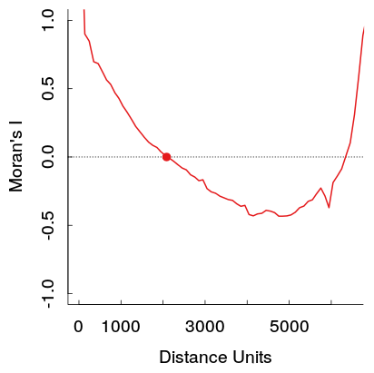
Moran’s I of the model residuals

Ideally Moran’s I should be as close to zero as possible. In the above plot you can see that values in close distance (up to 2000 Distance units) and with greater distance as well, the model residuals are positively autocorrelated (too great than expected by chance alone, thus correlated with proximity). The function correlog allows you to resample the dataset to investigate significance of this patterns, but for now i will just assume that our models residuals are significantly spatially autocorrelated.

There are numerous techniques to deal with or investigate spatial autocorrelation. Here the interested reader is advised to look at Dormann et al. (2007) for inspiration. In our example we will try to fit a simultaneous spatial autoregressive model (SAR) and try to see if we can partially get the spatial autocorrelation out of the residual error.  SARs can model the spatial error generating process and operate with weight
matrices that specify the strength of interaction between neighbouring sites (Dormann et al., 2007). If you know that the spatial autocorrelation occurs in the response variable only, a so called “lagged-response model” would be most appropriate, otherwise use a “mixed” SAR if the error occurs in both response and predictors. However Kissling and Carl (2008) investigated SAR models in detail and came to the conclusion that lagged and mixed SARs might not always give better results than ordinary least square regressions and can generate bias (Kissling & Carl, 2008). Instead they recommend to calculate “spatial error” SAR models when dealing with species distribution data, which assumes that the spatial correlation does neither occur in response or predictors, but in the error term.

So lets build the spatial weights and fit a SAR:

library(spdep)

x = xFromCell(amp,1:ncell(amp))
y = yFromCell(amp,1:ncell(amp))
z = getValues(amp)
nei <- dnearneigh(cbind(x,y),d1=0,d2=2000,longlat=T) # Get neighbourlist of interactions with a distance unit 2000.
nlw <- nb2listw(nei,style="W",zero.policy=T)
# You should calculate the interaction weights with the maximal distance in which autocorrelation occurs.
# But here we will just take the first x-intercept where positive correlation turns into the negative.
# Now fit the spatial error SAR
sar_e <- errorsarlm(z~topo,data=val,listw=nlw,na.action=na.omit,zero.policy=T)
# We use the generated z values and weights as input. Nodata values are excluded and zeros are given to boundary errors

# Now compare how much Variation can be explained
summary(fit1)$adj.r.squared # The r_squared of the normal regression
> 0.124
summary(sar_e,Nagelkerke=T)$NK # Nagelkerkes pseudo r_square of the SAR
> 0.504 # -- for SAR. So we could increase the influence of topographical average value on amphibian richness

# Finally do a likelihood ratio test
LR.sarlm(sar_e,fit1)
# Likelihood ratio for spatial linear models
>data:
>Likelihood ratio = 869.7864, df = 1, p-value &lt; 2.2e-16
>sample estimates:
>Log likelihood of sar_e; Log likelihood of fit1
> -7090.903 
>-7525.796

# Not only are our two models significantly different, but the log likelihood of our SAR is also greater than the ordinary model
# indicating a better fit.

The SAR is one of many methods to deal with spatial autocorrelation. I agree that the choice of of the weights matrix distance is a bit arbitrary (it made sense for me), so you might want to investigate the occurence of spatial correlations a bit more prior to fitting a SAR. So have we dealt with the autocorrelation? Lets just calculate Moran’s I values again for both the old residual and the SAR residual values. Looks better doesn’t it?

Comparison of Moran’s I for both a linear model and a error SAR residuals

References:

• F Dormann, C., M McPherson, J., B Araújo, M., Bivand, R., Bolliger, J., Carl, G., … & Wilson, R. (2007). Methods to account for spatial autocorrelation in the analysis of species distributional data: a review. Ecography, 30(5), 609-628.
• Kissling, W. D., & Carl, G. (2008). Spatial autocorrelation and the selection of simultaneous autoregressive models. Global Ecology and Biogeography, 17(1), 59-71.

Macroecology playground (2) – About the Mid domain effect null model

The use of null models in ecology has a long history (Connor & Simberloff,1979) and was in the epicenter of many scientific disputes. Some of them are even continuing until today (or here). I will spare the readers of this blog any further discussions or arguments as i haven’t entirely made up my own mind yet. Statistically speaking many null models make perfect sense for me if ecological data is just seen as “data”. The biological perspective of many null models however can be discussed as many of them make assumptions (random distribution of species in spatial community ecology for instance), which seem to be hardly true in natura. I agree that ecologists have to make careful considerations while designing their statistical analysis. I am going to follow the debate about null models more in the future, but for now let me introduce you to a simple null model in macroecology.

One of the most used null models in Macroecology is the so called Mid domain effect (MDE) null model. Given that the effect of all possible environmental predictors on a species distribution decreases, we would expect that the species richness peaks shift toward the center of their geometric constraints (Colwell & Lees, 2000; Colwell et al., 2004). This so called mid domain peak is build on the stochastic phenomena that if you shuffle species ranges inside a geometric constraint, you will always find that the greatest overlaps occur in the very center.
For an easy visualization: Just imagine an aluminum box full of different sized pencils. One of those you had back in primary school. The pencils inside are of varying size, some might be nearly as long as the whole box, others are nearly depleted. Close the box and shuffle it. If you now open the box again, you will find the most pencils (or parts of a pencil) in the middle of the box.

One way to generate a MDE null model from given species ranges is to use a so called spreading dye algorithm, which emulates grow of cells inside the given geometric constraints from a random starting point (emulating multiple drops of dye inside a water pont). Click the GIF image below to watch a growing MDE (CAREFUL – BIG GIF PICTURE > 4mb). As input the number of occupied grid cells per bird species in south America was used. The range was kept constant, but the starting point varies.

Click the image to see an animated .gif showing the developing MDE. CAREFUL – BIG GIF ON CLICK

As you can observe the relative bird species richness peaks in the middle of the continent after some time. This patterns becomes more prominent if the algorithm runs for all 2869 bird species occurring in south America. The final image and their range quartiles look like this :

Final result of a Mid domain model (relative richness and quartiles).

Here you can observe that the overall mid domain peak can only be observed for the fourth quartile. For the other three the relative distribution is quite random, which might explain why the MDE null model often explains quite a lot of the variance for widespread species (Dunn et al., 2007). The MDE null model has been criticized and defended again multiple times, but is still widely used in macroecology.  Critics usually bring up possible influences of phylogeny (Davies et al, 2005) or geometric constrains (Connolly, 2005; McClain et al., 2007). Issues particularly with the spreading dye algorithm are, that the simulated species ranges are like spreading ink drops which are very similar in shape. In reality species ranges often have quite complex and different configurations/shapes. Furthermore the models stops at the borders of the geometric contrains (the coastline of south America). Any random drop of ink near the coast line will therefore always grow into the heart of the country, which therefore makes the shape of the used geometric constrain the most important predictor of a possible range peak. If for instance the model would be repeated for a more irregular shape (like middle America) the peaks will develop where the greatest land mass is (so around texas and bolivia). The sheer probability of an ink dye developing in panama or Ecuador is too low due to the chance of hitting this small shape. This is a property of the algorithm and might result in non-significant null models for the middle American regions.

References

• Colwell RK, Lees DC (2000) The middomain effect: Geometric constraints on the
  geography of species richness. Trends Ecol Evol 15:70 –76.
• Colwell, R. K., Rahbek, C., & Gotelli, N. J. (2004). The Mid‐Domain Effect and Species Richness Patterns: What Have We Learned So Far?. The American Naturalist, 163(3), E1-E23.
• Connor, E. F., & Simberloff, D. (1979). The assembly of species communities: chance or competition?. Ecology, 1132-1140.
• Connolly, S. R. (2005). Process‐Based Models of Species Distributions and the Mid‐Domain Effect. The American Naturalist, 166(1), 1-11.
• Davies, T. J., Grenyer, R., & Gittleman, J. L. (2005). Phylogeny can make the mid-domain effect an inappropriate null model. Biology letters, 1(2), 143-146.
• Dunn, R. R., McCain, C. M., & Sanders, N. J. (2007). When does diversity fit null model predictions? Scale and range size mediate the mid‐domain effect. Global Ecology and Biogeography, 16(3), 305-312
• McClain, C. R., White, E. P., & Hurlbert, A. H. (2007). Challenges in the application of geometric constraint models. Global Ecology and Biogeography, 16(3), 257-264.

Macroecology playground (1) – Bird species richness in a nutshell

Ahh, Macroecology. The study of ecological patterns and processes on big scales.  Questions like “what factors determine distribution and diversity of all life on earth?” have troubled scientists since A.v.Humboldt and Wallace times. At the University of Copenhagen a whole research center has been dedicated to this specific field and macro-ecological studies are more and more present in prestigious journals like Nature and Science.  Previous studies at the center have found skewed distributions of bird richness with a specific bias towards the mountains (Jetz & Rahbek, 2002, Rahbek et al., 2007). In this blog post i am going to play a bit around with some data from Rahbek et al. (2007). The analysis and the graphs are by no means sufficient (and even violate many model assumptions like homoscedasticity, normality and data independence) and are therefore more of exploratory nature 😉 The post will show you how to build a raster stack of geographical data and how to use the data in some very basic models.

---

It was recommended to me to use the freely available SAM software for the analysis but although the program is really nice and fast it isn’t suitable enough for me as you can not modify specific model parameters or graphical outputs. And as a self-declared R junkie i refuse to work with “click-compute-result” tools 😉

So here is how the head of SAM data file  (“data.sam”)  looks like (i won’t share it, so please generate your own data).

As you can see the .sam file is technically just a tabulator separated table with the coordinates for a gridcell (1° gridcell on a latitude-longitude projection) and all response and predictor values for this cell. To get this data into R we are gonna use the raster package to generate a so called raster stack for our analysis. This is how i did it

# Load libraries
library(raster)
# Create Data from SAM
data <- read.delim(file="data.sam",header=T,sep="\t",dec=".") # read in a data.frame
coordinates(data) <- ~Longitude+Latitude # Convert to a SpatialPointsDataframe
cs <- "+proj=longlat +datum=WGS84 +no_defs" # define the correct projection (long-lat)
gridded(data) <- T # Make a SpatialPixelsDataframe
proj4string(data)  <- CRS(cs) # set the defined CRS

# Create Raster layer stack
s <- stack()
for(n in names(data)){
d <- data.frame(coordinates(data),data[,n])
ras <- rasterFromXYZ(xyz=d,digits=10,crs=CRS(cs))
s <- addLayer(s,ras)
rm(d,n,ras)
}
# Now you can query and plot the raster layers from the stack
plot(s$Birds.richness,col=rainbow(100,start=0.1))

South American Bird species Richness. Grain Size: 1°

You wanna do some modeling or extract data? Here you go. First we make a subset of some of our predictors from the raster stack and then fit ordinary least squares multiple regression models to our data to see how much variance can be explained. Note that linear regressions are not the proper techniques for this kind of analysis (degrees of freedom to high due to spatial autocorrelation, violation of assumptions mentioned before), but its still useful for explanatory purposes.

# Extract some predictors from the raster Stack
predictors <- subset(s,c(7,8,10))
names(predictors)
>  "NDVI" "Topographical.Range" "Annual.Mean.Temperature"
# Now extract the data from both the bird richness layer and the predictors
birds <- getValues(s$Birds.richness)
val <- as.data.frame(getValues(predictors))

# Do the multiple regression
fit <- lm(birds~.,data=val)
summary(fit)
>                          Estimate Std. Error t value Pr(>|t|)
(Intercept)             215.675282  15.837493   13.62   <2e-16 ***
NDVI                    -34.541242   1.245769  -27.73   <2e-16 ***
Topographical.Range       0.056458   0.002452   23.03   <2e-16 ***
Annual.Mean.Temperature   0.940664   0.054747   17.18   <2e-16 ***
---
Signif. codes:  0 ‘***’ 0.001 ‘**’ 0.01 ‘*’ 0.05 ‘.’ 0.1 ‘ ’ 1

Residual standard error: 81.86 on 1525 degrees of freedom
(1461 observations deleted due to missingness)
Multiple R-squared:  0.6931,    Adjusted R-squared:  0.6925
F-statistic:  1148 on 3 and 1525 DF,  p-value: < 2.2e-16

Ignore the p-values and just focus on the adjusted r² value. As you can see we are able to explain nearly 70% of the variance with this simple model. So how do our residuals and the predicted values look like? For that we have to create analogous raster layers containing both the predicted and the residual values. Then we plot all species raster layers again using the spplot function from the package sp (automatically loaded with “raster”)

# Estimates prediction
rval <- getValues(s$Birds.richness) # Create new values
rval[as.numeric(names(fit$fitted.values))]<- predict(fit) # replace all data-cells with predicted values
pred <- predictors$NDVI # make a copy of an existing raster
values(pred) <-rval;rm(rval) #replace all values in this raster copy
names(pred) <- "Prediction"

# Residual Raster
rval <- getValues(s$Birds.richness) # Create new values
rval[as.numeric(names(fit$residuals))]<- fit$residuals # replace all data-cells with residual values
resid <-predictors$NDVI
values(resid) <-rval;rm(rval)
names(resid) <- "Residuals"</pre>

# Do the plot with spplot
ss <- stack(s$Birds.richness, pred, resid)
sp <- as(ss, 'SpatialGridDataFrame')
trellis.par.set(sp.theme())
spplot(sp)

Multiple linear regression model output

While looking at the residual plot you might notice that our simple model fails to explain all the variation at mountain altitudes (the Andes).  Still the predicted values look very alike the observed richness. Bird species Richness is highest at tropical mountain ranges, which is consistent with results from Africa (Jetz & Rahbek, 2002). Reasons for this pattern are not fully understood yet, but if i had to discuss this with a colleague i would probably bring up arguments like older evolutionary time, higher habitat heterogeneity and greater numbers of climatic niches at mountain ranges. At this point you would then test for spatial autocorrelation using Moran´s I, adjust your data to that and use more sophisticated methods like General Additive Models (GAMs) or Spatial Autoregressive Model  (SARs) and account for the spatial autocorrelation. See Rahbek et al. (2007) for the actual study.

References:

• Jetz, W., & Rahbek, C. (2002). Geographic range size and determinants of avian species richness. Science, 297(5586), 1548-1551.
• Rahbek, C., Gotelli, N. J., Colwell, R. K., Entsminger, G. L., Rangel, T. F. L., & Graves, G. R. (2007). Predicting continental-scale patterns of bird species richness with spatially explicit models. Proceedings of the Royal Society B: Biological Sciences, 274(1607), 165-174.

Interesting Paper: Impact of Fragmentation on Plant-Frugivore networks redundancy

Jörg Albrecht, my former co-supervisor at the University of Marburg finally published his first results from his PhD. I was eagerly waiting for this publication as i also helped to raise a lot of data as a volunteer ornithologist while working on my bachelor thesis. Looking back i remember many nice beautiful moments like sitting in a camouflaged tent early in the morning counting frugivorous birds in the very core zone of Bialowieza forest. Bisons, Mooses, wildcats, the sound of howling wolfs in the morning were among the nice experiences i took with me. It was definitely a nice period of my life and i congratulate Jörg for publishing this nice paper! Published in the renown Journal of Ecology you can now access the paper in early-view:

Albrecht  et al. 2013 – Logging and forest edges reduce redundancy in plant–frugivore networks in an old-growth European forest

For those of you who want a little appetizer of what the paper is about. The paper itself incorporates information gained from many recently developed techniques for ecological network analysis to draw conclusions using general ecological theory (Optimal Foraging Theory). The optimal Foraging Theory developed by MacArthur (1955) hasn’t yet much appeared in the ecological network literature, which is a shame as it allows predictions about changing plant/animal specialization patterns in the light of habitat perturbations.  Here is a little summary, but i still recommend to read the full paper as both methods and conclusions are quite sophisticated 🙂

• 2 years of recorded plant-frugivorous interactions in Europe’s last old-growth lowland forest (Białowieza, Eastern Poland)
• Hypothesis (Summarized from the 3 expectations in the paper): Increased competition at Forest edges (caused by logging) compared to the interior forest leads to higher, respectively lower, redundancy in plant-frugivore networks. (But better read the paper!)
• To fully understand the extent of this study you need to dive deep into the study design and purpose. It uses state of the art statistical network-analysis techniques to calculate network redundancy and interaction specialization. Two and a half pages alone explain the data gathering and analysis, while the results sections is nearly half a page long 🙂
• Despite the small sample size (which was/is a major critical point) the results show that the networks redundancy was reduced at forest edges due to shifting dietary specialization of the interacting partners. As i remember from the data collection Black-caps and Blackbirds dominated in most of the assessed trees, which leads to an asymmetry in the interaction network. As shown in the paper this might be due to forest fragmentation.
• Possible Critic:The sampling effort of 10 studysites, which were sampled over 2 years might not be enough to detect real properties of ecological networks. However so far every study investigating ecological networks worked with incomplete data. I also don’t really trust the whole separation of species in specialist and generalists based on available literature. Although much is known up to now, both foraging and behavioral patterns of birds might change due to forest fragmentation and therefore such classification might be inaccurate depending on the study sites properties.
• Why is the study of interest?  Up to now not much is known about how temperate Plant-frugivore interactions change in the face of habitat perturbation. Most of the available literature was conducted in the tropics or didn’t incorporated whole interaction networks. Probably due to the geographical bias, most of the available literature furthermore failed to detect an effect on network stability as this study shows.

So, enough advertising 😉

Useful R functions for ecologists

Every biologist using R has some self-written functions he particularly likes and which are useful in many different analysis. Here i am sharing seven nifty functions, which have proven to be useful for me in the past. Many can be used in different contexts and their functionalities are certainly missing in the R base package.

# The function below uses the MASS package to fit provided values to given often used
# distributions. AIC and BIC information criterion values are calculated and returned in an ordered table
testdist <- function(values){
require(MASS)
distributions <- c("normal","lognormal","exponential","logistic","cauchy","gamma","geometric","weibull")
res <- data.frame(cbind(distributions)); res[,c("AIC","BIC")] <- NA
for(i in seq(1:nrow(res))){
fit <- fitdistr(values,densfun=as.character(res$distributions[i]),)
res$AIC[i] <- AIC(fit);res$BIC[i] <- BIC(fit)
}
res <- res[order(res$BIC,decreasing=F,na.last=T),]
return(res)
}
#Example output:
data(trees)
testdist(trees$Height)
#distributions AIC BIC
#weibull 204.6404 207.5083
#normal 205.7745 208.6425
#gamma 206.4929 209.3609
#lognormal 206.9348 209.8028
#logistic 207.0618 209.9298
#cauchy 218.2213 221.0893
#exponential 332.5055 333.9395
#geometric 332.5107 333.9447
# Those values shouldn't be taken for granted and you should always visually explore potential distributions
# for instance with histograms or qqplots !

# Standarderror of the mean (SEM)
stderr <- function(x) sqrt(var(x,na.rm=TRUE)/length(na.omit(x)))
#Example output:
stderr(trees$Height)
# > 1.144411

# Do segments on top of Scatter-Plot.
# Requires a transmitted data.frame with x-y values and a vector with line-length
doSegments <- function(x,y,ll,eps=0.05,...){
# Further Arguments are transmitted to segments
segments(x,y-ll,x,y+ll) # Build lines
segments(x-eps,y-ll,x+eps,y-ll) # Do the segments on top
segments(x-eps,y+ll,x+eps,y+ll) # and below
}
#Example output:
plot(trees$Girth,trees$Volume)
fit <- lm(trees$Volume~trees$Girth)
# Displays the residuals of a linear regression as errorbar
doSegments(trees$Girth,trees$Volume,ll=resid(fit) )

# Returns a list of the elements of x that are not in y
# and the elements of y that are not in x (not the same thing...)
setdiff2 <- function(x,y) {
Xdiff = setdiff(x,y)
Ydiff = setdiff(y,x)
list(X_not_in_Y=Xdiff, Y_not_in_X=Ydiff)
}
# Example output
a <- c("A","B","C","D")
b <- c("C","D","E","F")
setdiff2(a,b)
#> $X_not_in_Y
#> [1] "A" "B"
#> $Y_not_in_X
#> [1] "E" "F"

# Remove all NA-Values from a list
remNa <- function(x) {
return(subset(x,complete.cases(x)))
}
# Example Output
a <- c("A","B",NA,"D")
remNa(a)
#> [1] "A" "B" "D"

## String manipulation
# trim white space/tabs
trim_whitespace <-function(s) gsub("^[[:space:]]+|[[:space:]]+$","",s)

# Example output
a <- "   Teststring   "
trim_whitespace(a)
#> [1] "Teststring"

# Extract numbers from string or character
numbers_from_string <- function(x) as.numeric(gsub("\\D", "", x))

# Example output
a <- "We found 13 rabbits playing on the field"
numbers_from_string(a)
#> [1] 13